Cowell Propagation

This example demonstrates thecapabilities of AstroDynX’s numerical orbital propagation using Cowell’s method. The example compares different integration approaches and showcases JAX’s automatic differentiation for computing state transition matrices.

Key Features Demonstrated

Numerical Integration

• Cowell’s method for orbital propagation

• Event detection during integration

• J2 perturbation effects

JAX Capabilities

• Automatic differentiation for state transition matrices

• JIT compilation for performance optimization

• Vectorized operations for batch processing

Setup and Configuration

First, we import the necessary libraries and configure JAX for high precision computation. We also check the available devices for potential GPU acceleration.

%load_ext autoreload
%autoreload 2

from jax import numpy as jnp
import jax
from astrodynx import diffeq
import astrodynx as adx
from astrodynx import prop
from matplotlib import pyplot as plt

jax.config.update("jax_enable_x64", True)
jax.devices()

The autoreload extension is already loaded. To reload it, use:
  %reload_ext autoreload

[CudaDevice(id=0), CudaDevice(id=1)]

Cowell’s Method for Orbital Propagation

Orbital Dynamics

The above example demonstrates Cowell’s method for orbital propagation with the following key features:

• Force Models: We combine point mass gravity with J2 perturbations

• Event Detection: The integration automatically stops when the satellite altitude drops below a minimum radius

Cowell’s Method

Direct numerical integration of the equations of motion:

\[\frac{d^2\mathbf{r}}{dt^2} = -\frac{\mu}{r^3}\mathbf{r} + \mathbf{a}_{pert}\]

J2~J4 Perturbation

Earth’s oblateness effect:

\[\begin{split}\mathbf{a}_{J2} = -\frac{3\mu J_2 R_E^2}{2r^5}\begin{bmatrix} x(1 - 5 \frac{z^2}{r^2}) \\ y(1 - 5 \frac{z^2}{r^2}) \\ z(3 - 5 \frac{z^2}{r^2}) \end{bmatrix}\end{split}\]

\[\begin{split}\mathbf{a}_{J3} = -\frac{5\mu J_3 R_E^3}{2r^7}\begin{bmatrix} x(3 z - \frac{7 z^3}{r^2}) \\ y(3 z - \frac{7 z^3}{r^2}) \\ 6 z^2 - \frac{7 z^4}{r^2} - \frac{3}{5} r^2 \end{bmatrix}\end{split}\]

\[\begin{split}\mathbf{a}_{J4} = \frac{15\mu J_4 R_E^4}{8r^7}\begin{bmatrix} x(1 - \frac{14 z^2}{r^2} + \frac{21 z^4}{r^4}) \\ y(1 - \frac{14 z^2}{r^2} + \frac{21 z^4}{r^4}) \\ z(5 - \frac{70 z^2}{3 r^2} + \frac{21 z^4}{r^4}) \end{bmatrix}\end{split}\]

Event Detection

The integration stops when the satellite falls below the minimum radius.

\[r < r_{min}\]

def vector_field(t, x, args):
    acc = adx.gravity.point_mass_grav(t, x, args)
    acc += adx.gravity.j2_acc(t, x, args)
    acc += adx.gravity.j3_acc(t, x, args)
    acc += adx.gravity.j4_acc(t, x, args)
    return jnp.concatenate([x[3:], acc])


args = {"mu": 1.0, "rmin": 0.7, "J2": 1e-6, "J3": 1e-8, "J4": 1e-9, "R_eq": 1.0}

orbdyn = adx.prop.OrbDynx(
    terms=diffeq.ODETerm(vector_field),
    args=args,
    event=diffeq.Event(adx.events.radius_islow),
)

x0 = jnp.array([1.0, 0.0, 0.0, 0.0, 0.9, 0.0])

Propagate with Adaptive Steps

The solver uses adaptive time stepping for optimal accuracy and efficiency

t1 = 3.1

sol = prop.adaptive_steps(orbdyn, x0, t1)

ts = jax.device_get(sol.ts[jnp.isfinite(sol.ts)])
print(f"solution steps: {sol.ts.size}")
print(f"ts shape: {ts.shape}")

fig, ax = plt.subplots(figsize=(6, 4))
ax.plot(sol.ys[:, 0], sol.ys[:, 1], label="Trajectory")
circle = plt.Circle(
    (0, 0), radius=args["rmin"], color="lightgray", label=f"Min radius ({args['rmin']})"
)
ax.add_patch(circle)
ax.set_aspect("equal")
ax.set_xlim(-1.2, 1.2)
ax.set_ylim(-1.2, 1.2)
ax.legend()
ax.set_title("Propagated with Adaptive Steps")
plt.show()

solution steps: 4097
ts shape: (27,)

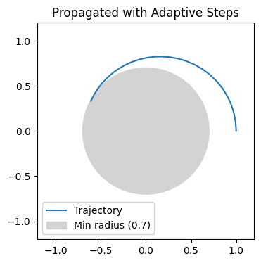
The trajectory shows the satellite’s path in the x-y plane, with the gray circle representing the minimum allowed altitude. The integration terminates when the satellite would impact this boundary.

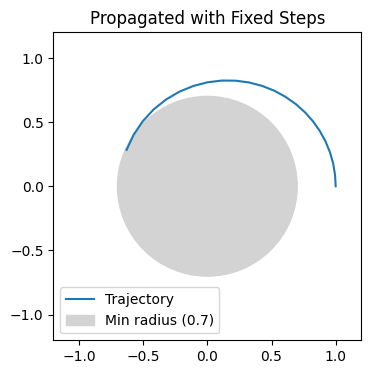
Propagate with Fixed Steps

dt = 0.1
sol = prop.fixed_steps(orbdyn, x0, t1, dt)
print(f"solution steps: {sol.ts.size}")
ts = jax.device_get(sol.ts[jnp.isfinite(sol.ts)])
print(f"ts shape: {ts.shape}")
step = jnp.mean(ts[1:] - ts[:-1])
print(f"step length: {step}")

fig, ax = plt.subplots(figsize=(6, 4))
ax.plot(sol.ys[:, 0], sol.ys[:, 1], label="Trajectory")
circle = plt.Circle(
    (0, 0), radius=args["rmin"], color="lightgray", label=f"Min radius ({args['rmin']})"
)
ax.add_patch(circle)
ax.set_aspect("equal")
ax.set_xlim(-1.2, 1.2)
ax.set_ylim(-1.2, 1.2)
ax.legend()
ax.set_title("Propagated with Fixed Steps")
plt.show()

solution steps: 4097
ts shape: (23,)
step length: 0.10000000000000003

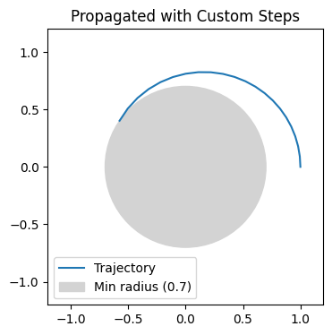
Propagate with Custom Steps

timesteps = jnp.linspace(0, t1, 32)
sol = prop.custom_steps(orbdyn, x0, t1, timesteps)
print(f"solution steps: {sol.ts.size}")
ts = jax.device_get(sol.ts[jnp.isfinite(sol.ts)])
print(f"ts shape: {ts.shape}")

fig, ax = plt.subplots(figsize=(6, 4))
ax.plot(sol.ys[:, 0], sol.ys[:, 1], label="Trajectory")
circle = plt.Circle(
    (0, 0), radius=args["rmin"], color="lightgray", label=f"Min radius ({args['rmin']})"
)
ax.add_patch(circle)
ax.set_aspect("equal")
ax.set_xlim(-1.2, 1.2)
ax.set_ylim(-1.2, 1.2)
ax.legend()
ax.set_title("Propagated with Custom Steps")
plt.show()

solution steps: 32
ts shape: (22,)

Propagate to Final Step

sol = prop.to_final(orbdyn, x0, t1)
print(f"final time: {sol.ts}")
print(f"final state: {sol.ys}")

final time: [2.15886367]
final state: [[-6.09055343e-01  3.33274544e-01  3.25637217e-08 -5.33368194e-01
  -1.18583962e+00  2.54194344e-08]]

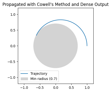
Dense Output

sol = prop.cowell_method(
    orbdyn, x0, t1, saveat=diffeq.SaveAt(dense=True, subs=diffeq.SubSaveAt(t1=True))
)

print(f"solution steps: {sol.ts[-1]}")
print(f"final state: {sol.ys[-1]}")
print(f"dense output at {sol.ts[-1]}: {sol.evaluate(sol.ts[-1])}")

fig, ax = plt.subplots(figsize=(6, 4))
ts = jnp.linspace(0, sol.ts[-1], 100)
ys = jax.vmap(sol.evaluate)(ts)
ax.plot(ys[:, 0], ys[:, 1], label="Trajectory")
circle = plt.Circle(
    (0, 0), radius=args["rmin"], color="lightgray", label=f"Min radius ({args['rmin']})"
)
ax.add_patch(circle)
ax.set_aspect("equal")
ax.set_xlim(-1.2, 1.2)
ax.set_ylim(-1.2, 1.2)
ax.legend()
ax.set_title("Propagated with Cowell's Method and Dense Output")
plt.show()

solution steps: 2.158863672875332
final state: [-6.09055343e-01  3.33274544e-01  3.25637217e-08 -5.33368194e-01
 -1.18583962e+00  2.54194344e-08]
dense output at 2.158863672875332: [-6.09055343e-01  3.33274544e-01  3.25637217e-08 -5.33368194e-01
 -1.18583962e+00  2.54194344e-08]

State Transition Matrix Computation

The above example demonstrates a powerful capability of JAX: computing exact derivatives through automatic differentiation. Here’s what happened:

1. Automatic Jacobian: jax.jacrev(yf)(x0) computes the Jacobian matrix \(\frac{\partial \mathbf{x}(t)}{\partial \mathbf{x}_0}\) automatically

2. Analytical Comparison: We compare against the analytical two-body solution to verify accuracy

3. High Precision: The results match to machine precision (1e-7 tolerance)

State Transition Matrix

The linearized dynamics around a reference trajectory:

\[\Phi(t, t_0) = \frac{\partial \mathbf{x}(t)}{\partial \mathbf{x}_0}\]

deltat = 2.5803148345055149
mu = 1.0

# initial state
r0_vec = jnp.array([-0.66234662571997105, 0.74919751798749190, -1.6259997018919074e-4])
v0_vec = jnp.array([-0.8166746784630675, -0.32961417380268476, 0.006248107587795581])

# final state
r_vec = jnp.array([-0.24986234273434585, -0.69332384278075210, 4.9599012168662551e-3])
v_vec = jnp.array([1.2189179487500401, 0.05977450696618754, -0.007101943980682161])

Verify the finnal state

def vector_field(t, x, args):
    acc = adx.gravity.point_mass_grav(t, x, args)
    return jnp.concatenate([x[3:], acc])


args = {"mu": mu}

orbdyn = adx.prop.OrbDynx(
    terms=diffeq.ODETerm(vector_field),
    args=args,
)

x0 = jnp.concatenate([r0_vec, v0_vec])
x1 = jnp.concatenate([r_vec, v_vec])
sol = prop.to_final(orbdyn, x0, deltat)
assert jnp.allclose(sol.ys[-1], x1, atol=1e-7)
r, v = prop.kepler(deltat, r0_vec, v0_vec, mu)
assert jnp.allclose(sol.ys[-1, :3], r[-1], atol=1e-7)
assert jnp.allclose(sol.ys[-1, 3:], v[-1], atol=1e-5)

Compute the State Transition Matrix

def yf(x, orbdyn, t1):
    return prop.to_final(orbdyn, x, t1).ys[-1]


jac_auto = jax.jacrev(yf)(x0, orbdyn, deltat)

jac_analytic = adx.twobody.dxdx0(r_vec, v_vec, r0_vec, v0_vec, deltat)
assert jnp.allclose(jac_auto, jac_analytic, atol=1e-7)